Modeling Epilepsy

TVB can be used to model large-scale epileptic seizure dynamics. Using relevant neural mass models, TVB allows to ask multiple questions such as the localisation of the epileptogenic zone or the validity of different neuroimaging modalities to assess the epileptogenicity of a brain structure. Here we will present an example of such a modelisation.

---

Objectives

The main goal of this tutorial is to provide a clear understanding of how we can reproduce clinically relevant senarios such as the modelisation of propagation of an epileptic seizure in the human brain, electrical stimulation of a brain region that can trigger a seizure, or surgical resection of brain regions.

In this project, all the data were already generated. You can download the ModelingEpilepsy.zip file in the TVB sharing area. We’ll only go through the necessary steps required to reproduce these simulations, along with the relevant outline. You can always start over, click along and/or try to change parameters. We will use the default subject connectivity matrix and surface.

---

Exploring the Epileptor model

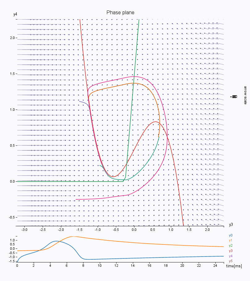
The Epileptor is a phenomenological neural mass model able to reproduce epileptic seizure dynamics such as recorded with intracranial EEG electrodes (see Jirsa_et_al). Before launching any simulations, we will have a look at the phase space of the Epileptor model to better understand its dynamics. We will use the phase plane interactive tool.

1. Go to simulator > > Phase plane and select the \(\mathbf{Epileptor}\) model.
2. Look at the phase space. We have here the first population (variables \(y_0\) in abscissa and \(y_1\) in ordinate). The left most intersection of the nullcline defines a stable fixed point, representing the interictal state, whereas the rightmost intersection is the center of a limit cycle, being the ictal state. Both states are separated by a separatrix, as you can se by drawing different trajectories in this phase space (left click on the figure).

3. You can also look at other variables in the phase space, such as the second population \(y_3\)/\(y_4\), responsible for the interictal spikes in the Epileptor model. Change the lower and upper bound of the axis to see correctly the phase space.

4. You can continue to play along to explore the dynamics of this model. For instance, try changing the number of integration steps, or choosing a HeunStochastic integrator and varying the scaling of the noise (parameter D).

---

Region-based modeling of a temporal lobe seizure

We will model temporal lobe epilepsy (TLE) using the Default TVB Subject. Here, using the tools in Set up Region model, we will set different values of epileptogenicity (\(x_0\) parameter in the Epileptor) according to the region positions, thereby introducing heterogeneities in the network parameters. We will set the right limbic areas (right hippocampus (rHC), parahippocampus (rPHC) and amygdala (rAMYG)) as epileptic zones. We will also add two lesser epileptogenic regions: the inferior temporal cortex (rTCI) and the ventral temporal cortex (rTCV).

1. First, we will configure the different parameter regimes we will use. Go on the Simulator page, click on the > Phase plane, in Parameter configuration name give the name Other Nodes, select the Epileptor model, set \(\mathbf{x_0=-2.4}\), and Save new parameter configuration on the right menu. Dynamic saved you should appear on the top right. Repeat the operation for an Epileptogenic zone with \(\mathbf{x_0=-1.6}\), and a Propagation zone with \(\mathbf{x_0=-1.8}\). Set \(\mathbf{R=0.00015}\). All the other model parameters are the default ones and are given in the following table.

Model parameter	Value
\(Iext\)	3.1
\(Iext2\)	0.45
\(slope\)	0.0

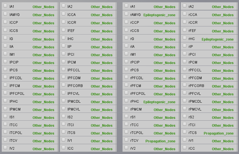
2. Now we will set up the different spatial configurations of these parameters. Go back to Simulator > Set up region Model, on the right of New selection, choose an name, such as Epileptogenic Zone and select the nodes rHC, rPHC, and rAMYG, then Save. You can use the button to go faster. Add also a Propagation Zone with the rTCI and rTCV nodes, and an Other Nodes selection with all nodes but rHC, rPHC, rAMYG, rTCI, and rTCV. You can use the button to go faster.
3. Now we will assign our parameter configurations to our spatial selections. In the same window, in Select model configuration select Epileptor - Epileptogenic Zone, select you precedent Epileptogenic Zone configuration, and click on Apply to selected nodes. A green label should appear on the right of the nodes assigned. Repeat the operation for the Propagation Zone and Other Nodes, then don’t forget to Submit Region Parameters on the right menu, which will bring you back to the Simulator panel. You can check that your choices have been save if you see a list of parameters in front of the X0 parameter for the Epileptor model.

4. We will now configure the simulation parameters. In the Simulator panel, choose a Difference Long-range coupling function with \(\mathbf{a=1.}\). We will add a permittivity coupling and a coupling on the time scale of spike-wave events. For this set \(\mathbf{K_s=-0.2}\) and \(\mathbf{K_f=0.1}\). Choose a HeunStochastic integration scheme, set the integration step size to 0.05 ms and an additive noise with \(\mathbf{D=[0., 0., 0., 0.0003, 0.0003, 0.]}\) (we add noise only on the second population).
5. For the monitors, we choose a Temporal average, an EEG and an Intracerebral / Stereo EEG monitor (hit CTRL to select several monitors). For all three Pre-monitor expressions, write \(mathbf{-y0+y3;y2}\) (this corresponds to first LFP signal, and second the slow dynamics of the Epileptor). Choose also the right Projection matrix, Region mapping and Sensors for each monitor, and a samplng period of 1 ms.
6. Choose a simulation length of 6000ms.
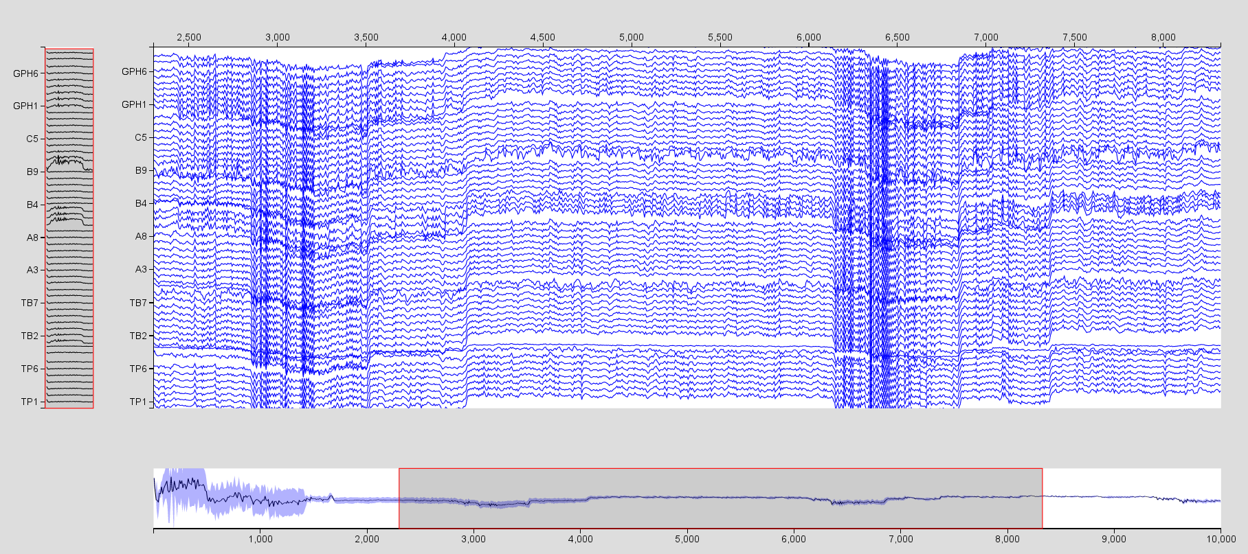
7. Configure View and add a Brain Visualizer. Save your choices.

The results are already computed for you in Region_TemporalLobe simulation.

8. Visualize the time series by clicking on the button. Click on Select Input Signals and select all the regions. From this same menu, you can select which state variables of interest will be displayed. For instance, visualize \(-y_0+y_3\). You will need to increase the scaling by clicking on . You can see a succession of 3 seizures, use the mouse to zoom in and out in the time series area.

9. Now click on , select the EEG time series, and Update the Visualizer. Chnage the scaling and the number of channels to see the seizures.

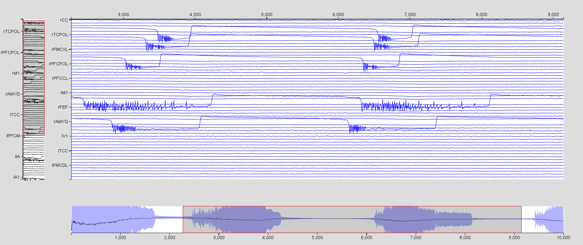
10. Repeat the operation for the SEEG time series, but select only the electrodes TB, A, B, C, and GPH which are in the right temporal lobe.

11. Go back to the Simulator page and visualize the results in the Brain Viewer, you will need to increase the rendering speed (timesteps per Frame) by clicking on .

The length of seizures here is not realistic (\(\sim 2\) s), but you can always obtain realistic time by multiplying all the derivatives of the model by a small factor.

---

Modeling surgical resection

Surgical resection is used for around 20% of epileptic patient whose seizures are drug- resistant. We will simulate the hypothetic case of a surgical resection of the amygdala and the hippocampus, but leaving the parahippocampal cortex.

1. Go to Connectivity > Large scale Connectivity. All nodes of the connectivity matrix are already selected.
2. Click on Q1 to go to Quadrant 4, and click on rAMYG and rHC to unselect these nodes. Give the name Resection at the right of Large Scale Matrix and save it by clicking on . Here we just created a new connectivity matrix while deleting all edges connected to the right amygdala and hippocampus.

3. Go back to Simulator and copy the Region_TemporalLobe simulation.
4. Choose the Resection connectivity matrix.
5. Go in Set up region model, and apply the dynamics of OtherNodes to rAMYG and rHC. (i.e. we replace the dynamics of the resected node by a stable node).

The results are given in resection_Region_TemporalLobe.

6. Click on Results, then TimeSeries and visualize the spatial average time series with the a Time Series visualizer. Don’t forget to increase the Scaling and Select all channels.

---

Triggering a seizure by stimulation

We are now going to model an electric stimulation and trigger a seizure. We set the whole brain to non-epileptogenic but close to the threshold

1. Go to stimulus > Region Stimulus
2. Give a name to the new stimulus
3. Choose a PulseTrain stimulation in time with parameters given in the following table:

Temporal parameters	Value
\(onset\)	2000.0
\(tau\)	20.0
\(T\)	4000.0
\(amp\)	10.0

4. Click on Set Region Scaling, select the Propagation Zone nodes, and apply a scaling of 1., and click on Save New Stimulus on Region in the right menu.

The stimulus was already set for you under the name Stim_PropagationZone

6. Go to simulator and copy the former simulation.
7. Choose the Stim_PropagationZone stimulus.

You can see the result of this simulation in stimulation_Region_TemporalLobe

8. Visualize the time series, zoom in to better see the effect of the stimulation.

---

More Documentation

For more information on the Epileptor model, see Jirsa_et_al, El_Houssaini_et_al, Proix_et_al, Naze_et_al .

---

Support

The official TVB webiste is www.thevirtualbrain.org. All the documentation and tutorials are hosted on http://docs.thevirtualbrain.org. You’ll find our public repository at https://github.com/the-virtual-brain. For questions and bug reports we have a users group https://groups.google.com/forum/#!forum/tvb-users

[Jirsa_et_al]

Jirsa VK, Stacey WC, Quilichini PP, Ivanov AI, Bernard, C. On the nature of seizure dynamics. Brain, 2014. 137:2210-2230

[El_Houssaini_et_al]

El Houssaini K, Ivanov A, Bernard C, Jirsa VK. Seizures, refractory status epilepticus, and depolarization block as endogenous brain activities. Physical Review E, 2015; 91:2-6

[Proix_et_al]

Proix T, Bartolomei F, Chauvel P, Bernard C, Jirsa VK. Permittivity Coupling across Brain Regions Determines Seizure Recruitment in Partial Epilepsy. The Journal of Neuroscience, 2014; 34:15009-15021

[Naze_et_al]

Naze S, Bernard C, Jirsa VK. Computational Modeling of Seizure Dynamics Using coupled Neuronal Networks: Factors Shaping Epileptiform Activity. PLOS CB, 2015, 11